Our interest in exploring OpenCL came from a customer who wished to accelerate their image processing on a CPU (NXP i.MX8MN) that doesn’t include a dedicated Image Signal Processing (ISP) engine to perform the task. So a software route is the only option. NXP themselves provide a simple toolkit (SoftISP), but it is rather limited by being tied into their demo environment and being fixed in terms of image size and ease of use. So it was decided to have a look from first principles.
It was around 12 years ago that OpenCL came onto the scene, initially via demos from Apple, AMD and NVIDIA which quickly lead into full Software Development Kits being released for those platforms. The premise was to extend the accessibility of the parallel processing ability of GPUs (already accessed via OpenGL) and to open it up to more general compute tasks. By presenting a more general API it allows for a back-end agnostic approach, which has allowed FPGAs and other “accelerators” to be utilised.
GPU’s however make up the bulk of the usage. Almost every modern GPU with a 3D rendering pipeline has an OpenCL support layer. Their wide memory busses and highly paralleled (and often vectorised) processing engines lend themselves to the kinds of tasks where the same operation needs to be carried out on large, mostly independent, data sets. It’s interesting to note that the highest end GPUs are used on cards with no video output paths, they are used purely for their processing power (AMD Instinct, NVIDIA Datacenter GPUs etc.)
OpenCL, and a lot of the other related standards, are under the stewardship of the Khronos Group. A industry body supported by almost all of the top hardware and software bodies who have an interest in these topics. As such access to the OpenCL standard and documentation is free and easily accessible.
An embedded GPU might not have the thousands of processing elements that a top specification GPU from AMD or NVIDIA has but it has much of the same basic structure. Consisting of a small number of Compute Elements each with a number of processing units, local memory/registers with fast access, L1 Cache and access to a more global memory etc. Generally this is the same hardware that performs Texture and Pixel processing when used for 2D/3D graphics. Taking, for example, the popular NXP i.MX8 series which contain members of the Vivante 7000 series GPU family – the number of processing units range from 8 to 32, while clock speeds range from 400 to 1000Mhz across different models. Admittedly nothing spectacular when compared to, say, an NVIDIA Ampere. But the i.MX8+GPU may well be <5W at full power, where as Ampere based system is well past 350W for just the GPU alone, and would need something like an additional 200W CPU feeding it data at the very least. They are designed to operate in entirely different market segments.
Lets examine one of the reasonably common image processing tasks, namely debayering/demosaicing data captured from a CCD camera. The way a CCD works means you do not get RGB values for each pixel. Instead it generally looks like a mosaic of pixel in a 2×2 repeating pattern. (There are in general 4 main encoding schemes used, although different manufactures do have some more exotic ones. The abundance of green pixels is to better match the human eye’s sensitivity to those wavelengths.)

This needs to be processed to obtain a familiar RGB image we are all used to using. You can do this in a variety of ways, with a variety of algorithms. There are trade offs between speed and quality for each. Simple fast methods often produce artefacts due to the offset nature of the pixels. One of the more popular high quality ways to perform the processing is the Malvar-He-Cutler method. This does sub-sampling of neighbouring pixels using a specific patterns, with differing weights per pixel, to calculate the missing component at the pixel in question. E.g. on Green pixels you need to calculate the R and B channel components. The general operation works on a 5×5 pixel area to calculate the resulting pixel (These patterns as known as Cross, Phi, Theta and Checker).
From the original published paper published in 2004 these are:

Taking these patterns and knowing that for every pixel in the image these operations need to be performed it becomes very attractive to use a massively parallelised method to do the operation. The input data is constant, all the outputs are independent of each other and the operation per pixel is identical to a first approximation. GPUs become very attractive for performing the task.
While direct hardware programming would allow the most performance to be obtained it presents far too many problems with regards to portability, interacting with the Operating System, allocating memory, transferring between virtual and physical addresses and dealing with the fact the GPU may need to be multiplexed with other tasks such as 3D graphics, Display rendering or other applications trying to do the same thing.
OpenCL backs off just enough from the hardware level and presents a way to use a modified C/C++ dialect to perform the programming and then a support structure around this to handle the allocation of buffers, data transfers, signalling and a host of other high level operations. All in a mostly portable way. With this, the same code can be run on the 300W NVIDIA GPU as the 5W NXP i.MX8 one.
The 1.2 OpenCL specification is well supported across all manufactures (2.2 is also popular and 3.0, although the most recent is rapidly being supported). All versions have the same basic concepts.

A Platform (NVIDIA, AMD, NXP etc) can have multiple Devices (GPUs for instance, or even DSP and CPU) under it. These execute the Program/Kernel via a Command Queue. Everything is tied together using a Context which acts as the main programming handle to ensure everything is kept consistent.
The basic flow is to query for Platforms, then Devices under those platforms that you want to use.
cl_int errCode;
cl_uint totalPlatforms = 0;
cl_uint totalDevices = 0;
cl_platform_id platform = 0;cl_device_id device = 0;

errCode = clGetPlatformIDs(1, &platform, &totalPlatforms);
errCode = clGetDeviceIDs(platform, CL_DEVICE_TYPE_GPU, 1, &device, &totalDevices);
Providing the ones you want are available you create a Context that binds them together.
cl_context context = clCreateContext(NULL, 1, &device, NULL, NULL, &errCode);You create a Command Queue to allow work to be performed on the device.
// The queue can execute work out of order (Only useful there are no dependencies)
cl_command_queue_properties queue_props = CL_QUEUE_OUT_OF_ORDER_EXEC_MODE_ENABLE;

cl_command_queue queue = clCreateCommandQueue(context, device, queue_props, &errCode);
You compile (at runtime) the OpenCL code (or assemble it from pre-compiled fragments) and create the Kernel that will be executed. Code can be read from the file system or included as text inside your host side executable.
// NOTE: Pre-read source code into the Buffer before passing to
// OpenCL for compiling if reading from the filesystem.
// File/buffer can be free'd after build.

program = clCreateProgramWithSource(ctx, 1,
                 (const char**)&programBuffer, &programSize, &clErr);

// Compile options are like normal CFLAGS, with -D <something> -I <path> etc.
// Include file and paths are respected.
// There are often architecture specific optimisation flags
clErr = clBuildProgram(program, 0, 0, compileOptions, 0, 0);

// Convert into a Kernel that can be executed
kernel = clCreateKernel(Program, KERNEL_FUNC, &errCode);
Some OpenCL implementations offer methods via environmental flags to display compiler output on the terminal as it processes. There is also an explicit OpenCL function to obtain the information such as the logs (clGetProgramBuildInfo). There is the ability to load pre-compiled platform dependent binaries (clCreateProgramWithBinary) and an intermediate platform independent pre-compiled format known as SPIR-V also exists in OpenCL 2.2 (clCreateProgramWithIL).
Data needs to be transferred to and from the OpenCL device. Usually you are working in one or more input buffers with one or more output buffers for the results. This is done with Buffer/Image objects. To aid with optimisation you can specify the direction of the buffers and this may improve performance on some operating systems.
inputCLBuffer = clCreateBuffer(context,                     CL_MEM_READ_ONLY |CL_MEM_HOST_WRITE_ONLY,
                    frameInSize, 0, &errCode); // <=====INPUT Buffer

outputCLBuffer = clCreateBuffer(context,
                     CL_MEM_READ_WRITE |CL_MEM_HOST_READ_ONLY,
                     frameOut, 0, &errCode); // <=====OUTPUT Buffer
It is possible to pass the input data through at buffer creation time and have the OpenCL use the Host’s already allocated memory, but there are alignment issues that need to be considered if that option is taken. If those can be accommodated it can allow zero copy operation. The other option is to write into the buffer after creation but before executing the kernel.
// Direct write into a buffer
clErr = clEnqueueWriteBuffer(queue, inputCLBuffer,
                 CL_TRUE, inputOffset, frameSize,
                 (void *)data, 0, 0, 0);

// Alternative, similar to mmap(), allows you to directly access
// the memory itself. Remember to unmap!
address = (uint8_t *)clEnqueueMapBuffer(queue,
                       inputCLBuffer, CL_TRUE,
                       CL_MAP_WRITE, 0, frameSize,
                       0,NULL, 0, &clErr);

// Do you operations here, e.g. read() into it from file
read(fd, address, frameSize);
// Unmap
clErr = clEnqueueUnmapMemObject(queue, inputCLBuffer,                      address, 0, NULL, NULL);
Arguments can be set for the Kernel (just like a C function call). It will check on execution that they match the prototype given. Arguments are copied, so the temporary variable can be reused.
cl_uint tmp = bufferHeight;
clSetKernelArg(kernel, 0, sizeof(cl_uint), &tmp);
tmp = bufferWidth;
clSetKernelArg(kernel, 1, sizeof(cl_uint), &tmp);
clSetKernelArg(kernel, 2, sizeof(cl_mem), &inputCLBuffer);
Finally it can be executed. You specify an array that describes the data size and how you want it split up. This is multi-dimensional, however quite often things are 2D so the third is ignored/assumed to be 1. As it is running on a separate processor you need to synchronise things in order to know when the operation is done. So execution waits for the OpenCL queue to finish.
// We process 4 pixels in x, and 2 rows in y per work item
size_t global_work_size[2] = {bufferHeight/2, bufferWidth/4};

// local work size is how the global size is split up, and can
// be related to the hardware's internal structure.
size_t local_work_size[2] = {5,8};

errCode = clEnqueueNDRangeKernel(queue, kernel, 2, NULL,                 (const size_t*)&global_work_size,
                (const size_t*)&local_work_size,
                0, NULL, NULL);

// Wait for it to finish
errCode = clFinish(queue);
Data can then be retrieved from the buffers. Again, this can be via mapping the buffer or a direct read command (clEnqueueReadBuffer).
address = (uint8_t *)clEnqueueMapBuffer(queue, outputCLBuffer,
                     CL_TRUE, CL_MAP_READ, 0, frameOutSize,
                     0,NULL, 0, &clErr);

// Write to file directly from buffer
write(fd, address, frameOutSize);

// unmap
clErr = clEnqueueUnmapMemObject(queue, outputCLBuffer, address, 0, NULL, NULL);
Now, the above methodology is rather linear and not ideal for performance in a multi threaded environment. However OpenCL comes with the concept of Events, and these can be set up such that steps can be made dependent on each other, and callback hooks can be implemented. This allows for operations to be streamlined and parallelised even more with read, write and processing threads. For a bit more information see https://ece.northeastern.edu/groups/nucar/Analogic/Class5-B-Events.pdf
So far we’ve looked at the Host/CPU side – let’s now consider the OpenCL/GPU side. Back when the Kernel was created with clCreateKernel() a function name was specified. This is the entry point in the OpenCL code and is qualified with __kernel.
// This version takes a tile (z=1) and each tile job does 4x2 pixels
// Workgroup size is passed in at build time as a MACRO.
//
// _global qualifier means the buffer is in global memory
 attribute((reqd_work_group_size(TILE_COLS, TILE_ROWS, 1)))
 __kernel void malvar_he_cutler_demosaic(const uint im_rows, const uint im_cols,
         __global const uchar input_image_p, const uint input_image_pitch,
         __global uchar *output_image_p, const uint output_image_pitch,
         const int bayer_pattern, const int add_border) {
// C-code for the kernel...
}
In the kernel you have access to a variety of system function calls and standard operations. Some of these calls allow you to get the position in the global work, as well as the local work location. In a pixel based operation these can be used to work out where you are in the buffer for instance.
// Get our location in the buffer/image
const uint g_col = get_global_id(0)*4; // Doing 2 columns at a time in Column/x dim
const uint g_row = get_global_id(1)*2; // Doing 2 rows at a time in Row/y dim
One of the main things to remember is that most OpenCL code will be running on processors that are adapted to vector operations with very wide registers and data paths. There are vector versions of almost all the standard data types and making use of these can bring substantial speed increases on some architectures. The most efficient width can often be found in the documentation for the hardware or via clGetDeviceInfo(). Some compilers are better than others at converting the code into vector operations so it often pays to do the work by hand.
Data loading from global memory to local is also usually more efficient when done as a vector. This is often due to cache line lengths and other internal data paths. vload() comes in 2, 4, 8 and 16 object sizes, and all supported data types. There are memory alignment considerations to be aware of however with these.
// Load 8 lines of 8 pixels.
// Compiler will determine if LineX becomes a register or fast local memory.
    lineA = vload8(0, (uchar *)(psrc + line_offsetA));    lineB = vload8(0, (uchar *)(psrc + line_offsetB));
    lineC = vload8(0, (uchar *)(psrc + line_offsetC));
    lineD = vload8(0, (uchar *)(psrc + line_offsetD));
    lineE = vload8(0, (uchar *)(psrc + line_offsetE));
    lineF = vload8(0, (uchar *)(psrc + line_offsetF));
The components of the vector can then be accessed in a similar way to a data structure. For simple vectors the usual terminology is to use letters (xyzw), however as vectors get bigger a lot of code switches to numbers prefixed with sN for each location. (s0123 etc.)
// Access vector using .sN notation
float4 Dvec = (float4)(lineB.s1, lineD.s1, lineB.s3, lineD.s3);

// Access vector using .xyzw notation
// Code sums the vector into .x
Dvec.xy += Dvec.zw;
Dvec.x  += Dvec.y;
More complicated examples can take advantage of the fact you can repeat the vector access index, or re-order them to swap byte orders. Often with very little penalty in terms of performance. An example of this, going back to the debayering problem, is calculating all 4 possible pixel patterns at the same time. The symmetry of these means it can be factored down to a few vector operations with multiplication co-efficient values. Pixels are shared across pattern with differing co-efficient values.
 // Centre pixel coefficients
 const float4 kC = (float4)( 4.0/8.0,  6.0/8.0,  5.0/8.0,  5.0/8.0);

 // Pattern pixel coefficients
 const float4 kA = (float4)(-1.0/8.0, -1.5/8.0,  0.5/8.0,  -1.0/8.0);
 const float4 kB = (float4)( 2.0/8.0,  0.0,      0.0,       4.0/8.0);
 const float4 kD = (float4)( 0.0,      2.0/8.0, -1.0/8.0,  -1.0/8.0);

 // const float4 kE = (float4)(-1.0/8.0, -1.5/8.0, -1.0/8.0    0.5/8.0);
 // const float4 kF = (float4)( 2.0/8.0,  0.0,      4.0/8.0    0.0    );
 // Use a load from the other registers, with a "swizzle", it's the same
 // or faster
 const float4 kE = kA.xywz;
 const float4 kF = kB.xywz;

 // Center pixel * its coefficient
 float4 PATTERN = (kC.xyz * lineC.s2).xyzz;

 // Square around centre pixel, +/- 1 in x/y
 float4 Dvec = (float4)(lineB.s1, lineD.s1, lineB.s3, lineD.s3);

 // Upper Vertical and Left Horizontal pixels
 float4 value = (float4)(lineA.s2, lineB.s2,  lineC.s0, lineC.s1);

 // Lower Vertical and Right Horizontal pixels
 float4 temp = (float4)(lineE.s2, lineD.s2,  lineC.s4, lineC.s3);

 // Sum Square pixel block
 Dvec.xy += Dvec.zw;
 Dvec.x  += Dvec.y;

 // Sum the Vertical and Horizontal pixels.
 value += temp;

 // Add square (multiplied by coefficients)
 PATTERN.yzw += (kD.yz * Dvec.x).xyy;

 // Add in the vertical and horizontal parts for each patter.
 PATTERN += (kA.xyz * (float3)(value.x,value.x,value.x)).xyzx +
            (kE.xyw * (float3)(value.z,value.z,value.z)).xyxz;
 PATTERN.xw  += kB.xw * (float2)(value.y,value.y);
 PATTERN.xz  += kF.xz * (float2)(value.w,value.w);
 // PATTERN now contains all 4 possible combinations for that pixel position.
The value for the pixel RGB is now just the actual current pixel value and the correct pattern combinations to calculate the other two channels. These depend on the Bayer pattern type and the position of the pixel inside the 2×2 grid. By repeating the above calculations and offsetting the pixel by +1 horizontally each time you can quickly calculate 4 adjacent values.
Data writes back to global memory are often more efficient if done in a vector access as well. So there are matching vstore() functions to handle this. An alpha channel is added, and set to maximum as it is easier to work with data that is by 4 rather than by 3 wide.
// rgb4 is a vector which is 4*RGBA Pixels (16 bytes total)
// out_offset is the calculated base pixel offset into the output
vstore16(rgb4, 0 , (uchar *)(output_image_p+out_offset));
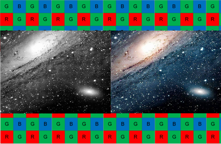
Original Image on the left, processed on the right.
On the lowest i.MX8 (2 CU with 4 Compute Elements each) the OpenCL was able to work at a rate of ~32Mpixels/sec, leaving the quad core CPU free to perform other operations in the image processing pipeline.
For comparison the same code running on a NVIDIA GTX 1650 Ti (16 CU with 64 Compute Elements each) delivers ~3200Mpixels/sec.
The important thing to consider is that while pretty much all OpenCL kernels will run on complaint OpenCL hardware they may not deliver the highest performance possible. Each hardware manufacture has their own suggestions for optimisations across their architectures. Often related to the number of parallel work items, how they access memory (Registers vs Local vs Shared), best sizes for any vectors and even some replacement OpenCL extensions that can provide performance improvements.
Profiling tools are usual available for most systems if there is a need to squeeze out the last drops of performance, however as with a lot of things on an Embedded system these are often not so straight forward to obtain or utilise.
One interesting result of this work was that whilst performance on a mid to high end desktop GPU was impressive, on an embedded platform it could be easily outperformed by using tuned ARM Neon based implementations – one of the most efficient is bayer2rgb by Enrico Scholz. It is a trade-off between CPU usage and time. On a Quad core embedded system it can possibly be more efficient overall to use a CPU core for the task depending on how demanding the application is and where bottlenecks are.
The OpenCL code was inspired by:
- NXP SoftISP https://github.com/NXPmicro/gtec-demo-framework/tree/master/DemoApps/OpenCL/SoftISP
- OpenCL Examples provided by GrokImageCompression https://github.com/GrokImageCompression/latke
A good overview of OpenCL is provided by Khronos at https://github.com/KhronosGroup/OpenCL-Guide. They also provid other tools and useful information on their github.
Reference cards for the different revisions of the specification are available here:
- 1.2 https://www.khronos.org/registry/OpenCL//sdk/1.2/docs/OpenCL-1.2-refcard.pdf
- 2.2 https://www.khronos.org/files/opencl22-reference-guide.pdf
- 3.0 https://www.khronos.org/files/opencl30-reference-guide.pdf
Finally, more information about the SoftISP and its performance can be found in this whitepaper.